Aarts, E., Dolan, C. V., Verhage, M., and Sluis, S. van der (2015),
“Multilevel analysis quantifies variation in the experimental effect while optimizing power and preventing false positives,” BMC Neuroscience, 16, 94.
https://doi.org/10.1186/s12868-015-0228-5.
Barr, D. J. (2013),
“Random effects structure for testing interactions in linear mixed-effects models,” Frontiers in Psychology, 4, 328.
https://doi.org/10.3389/fpsyg.2013.00328.
Bates, D., Mächler, M., Bolker, B., and Walker, S. (2015),
“Fitting Linear Mixed-Effects Models Using lme4,” Journal of Statistical Software, 67, 1–48.
https://doi.org/10.18637/jss.v067.i01.
Bolker, B. M., Brooks, M. E., Clark, C. J., Geange, S. W., Poulsen, J. R., Stevens, M. H. H., and White, J.-S. S. (2009),
“Generalized linear mixed models: A practical guide for ecology and evolution,” Trends in Ecology & Evolution, 24, 127–135.
https://doi.org/10.1016/j.tree.2008.10.008.
Brown, V. A. (2021),
“An Introduction to Linear Mixed-Effects Modeling in R,” Advances in Methods and Practices in Psychological Science, 4, 2515245920960351.
https://doi.org/10.1177/2515245920960351.
Casals, M., Girabent-Farrés, M., and Carrasco, J. L. (2014),
“Methodological quality and reporting of generalized linear mixed models in clinical medicine (2000-2012): A systematic review,” PloS One, 9, e112653.
https://doi.org/10.1371/journal.pone.0112653.
Galecki, A. T., Kathleen B. Welch (2014),
Linear Mixed Models: A Practical Guide Using Statistical Software, Second Edition, New York: Chapman; Hall/CRC.
https://doi.org/10.1201/b17198.
GRUEBER, C. E., NAKAGAWA, S., LAWS, R. J., and JAMIESON, I. G. (2011),
“Multimodel inference in ecology and evolution: Challenges and solutions,” Journal of Evolutionary Biology, 24, 699–711. https://doi.org/
https://doi.org/10.1111/j.1420-9101.2010.02210.x.
Harrison, X. A., Donaldson, L., Correa-Cano, M. E., Evans, J., Fisher, D. N., Goodwin, C. E. D., Robinson, B. S., Hodgson, D. J., and Inger, R. (2018),
“A brief introduction to mixed effects modelling and multi-model inference in ecology,” PeerJ, 6, e4794.
https://doi.org/10.7717/peerj.4794.
Jolly, E. (2018),
“Pymer4: Connecting R and Python for Linear Mixed Modeling,” Journal of Open Source Software, 3, 862.
https://doi.org/10.21105/joss.00862.
Lee, Y.-C., and Shang, J. (n.d.),
“Estimation and selection in linear mixed models with missing data under compound symmetric structure,” Journal of Applied Statistics, 49, 4003–4027.
https://doi.org/10.1080/02664763.2021.1969342.
Magezi, D. A. (2015),
“Linear mixed-effects models for within-participant psychology experiments: An introductory tutorial and free, graphical user interface (LMMgui),” Frontiers in Psychology, 6, 2.
https://doi.org/10.3389/fpsyg.2015.00002.
Marjolein Fokkema, J. E.-C., and Wolpert, M. (2021),
“Generalized linear mixed-model (GLMM) trees: A flexible decision-tree method for multilevel and longitudinal data,” Psychotherapy Research, Routledge, 31, 329–341.
https://doi.org/10.1080/10503307.2020.1785037.
Monsalves, M. J., Bangdiwala, A. S., Thabane, A., and Bangdiwala, S. I. (2020),
“LEVEL (Logical Explanations & Visualizations of Estimates in Linear mixed models): Recommendations for reporting multilevel data and analyses,” BMC Medical Research Methodology, 20, 3.
https://doi.org/10.1186/s12874-019-0876-8.
Peng, H., and Lu, Y. (2012),
“Model selection in linear mixed effect models,” Journal of Multivariate Analysis, 109, 109–129.
https://doi.org/10.1016/j.jmva.2012.02.005.
Piepho (1999),
“Analysing disease incidence data from designed experiments by generalized linear mixed models,” Plant Pathology, 48, 668–674. https://doi.org/
https://doi.org/10.1046/j.1365-3059.1999.00383.x.
Pusponegoro, N. H., Rachmawati, R. N., Notodiputro, K. A., and Sartono, B. (2017),
“Linear Mixed Model for Analyzing Longitudinal Data: A Simulation Study of Children Growth Differences,” Procedia Computer Science, Discovery and innovation of computer science technology in artificial intelligence era:
The 2nd
International Conference on
Computer Science and
Computational Intelligence (
ICCSCI 2017), 116, 284–291.
https://doi.org/10.1016/j.procs.2017.10.071.
Schielzeth, H., Dingemanse, N. J., Nakagawa, S., Westneat, D. F., Allegue, H., Teplitsky, C., Réale, D., Dochtermann, N. A., Garamszegi, L. Z., and Araya-Ajoy, Y. G. (2020),
“Robustness of linear mixed-effects models to violations of distributional assumptions,” Methods in Ecology and Evolution, 11, 1141–1152. https://doi.org/
https://doi.org/10.1111/2041-210X.13434.
Steibel, J. P., Poletto, R., Coussens, P. M., and Rosa, G. J. M. (2009),
“A powerful and flexible linear mixed model framework for the analysis of relative quantification RT-PCR data,” Genomics, 94, 146–152.
https://doi.org/10.1016/j.ygeno.2009.04.008.
Touraine, C., Cuer, B., Conroy, T., Juzyna, B., Gourgou, S., and Mollevi, C. (2023),
“When a joint model should be preferred over a linear mixed model for analysis of longitudinal health-related quality of life data in cancer clinical trials,” BMC medical research methodology, 23, 36.
https://doi.org/10.1186/s12874-023-01846-3.
Tu, Y.-K. (2015),
“Using generalized linear mixed models to evaluate inconsistency within a network meta-analysis,” Value in Health, 18, 1120–1125. https://doi.org/
https://doi.org/10.1016/j.jval.2015.10.002.
Verbeeck, J., Faes, C., Neyens, T., Hens, N., Verbeke, G., Deboosere, P., and Molenberghs, G. (2023),
“A linear mixed model to estimate COVID-19-induced excess mortality,” Biometrics, 79, 417–425.
https://doi.org/10.1111/biom.13578.
Wang, X., Andrinopoulou, E.-R., Veen, K. M., Bogers, A. J. J. C., and Takkenberg, J. J. M. (2022),
“Statistical primer: An introduction to the application of linear mixed-effects models in cardiothoracic surgery outcomes research-a case study using homograft pulmonary valve replacement data,” European Journal of Cardio-Thoracic Surgery: Official Journal of the European Association for Cardio-Thoracic Surgery, 62, ezac429.
https://doi.org/10.1093/ejcts/ezac429.
Zuur, A. F., and Ieno, E. N. (2016),
“A protocol for conducting and presenting results of regression-type analyses,” Methods in Ecology and Evolution, 7, 636–645. https://doi.org/
https://doi.org/10.1111/2041-210X.12577.
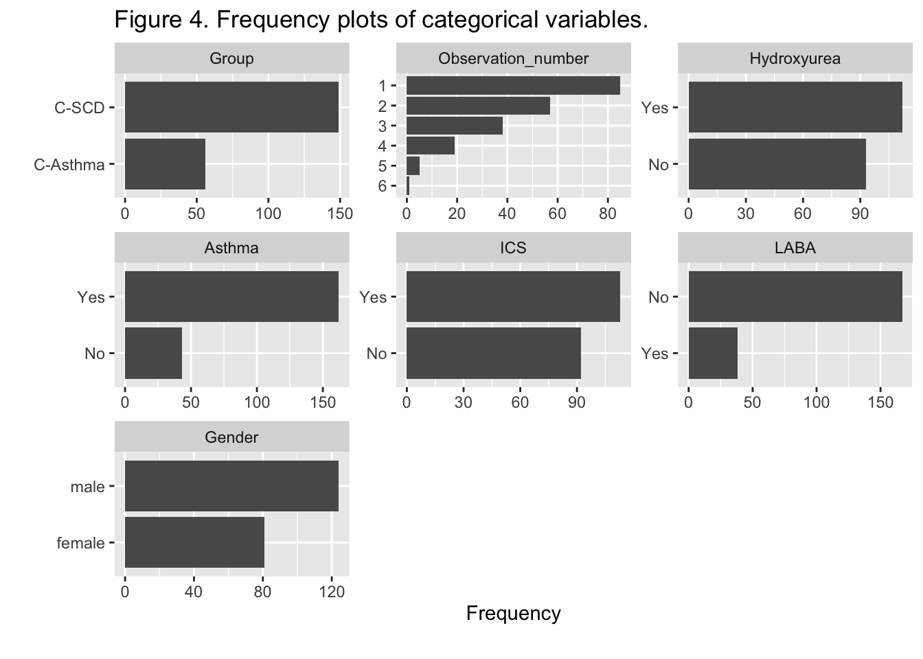
 {.lightbox}
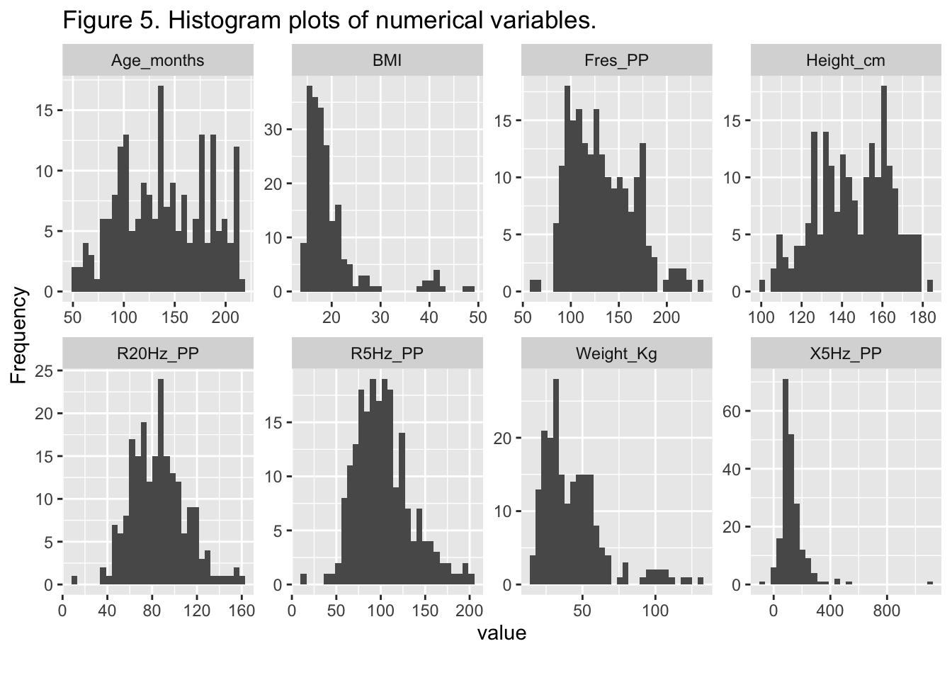
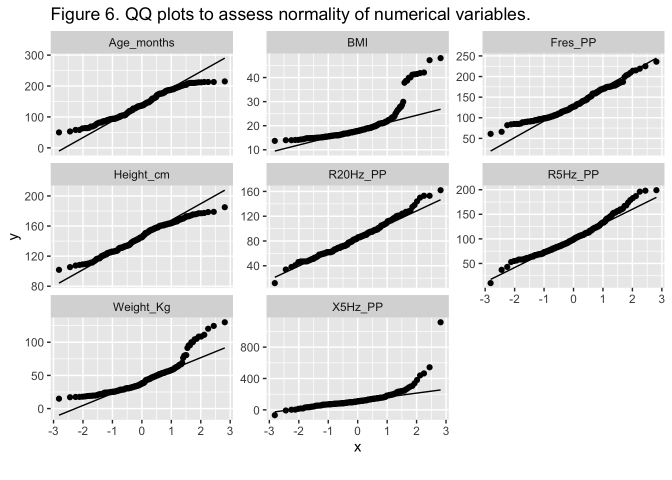
 {.lightbox}
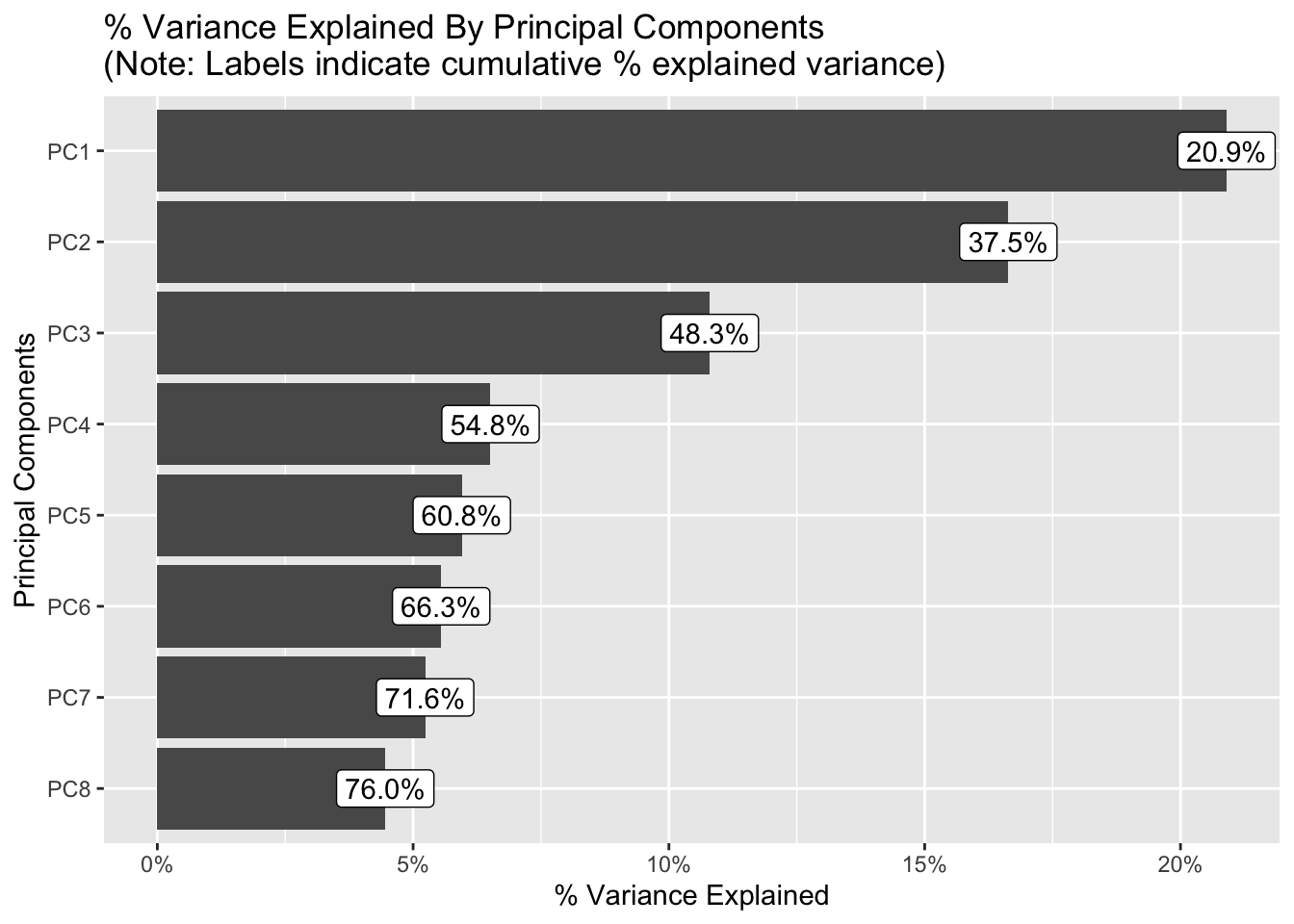